This notebook is the jupyter version of the streamlit app. It should use the same base data set but perhaps perform different calculations to iterate more quickly than on streamlit.
Code
import pandas as pdimport numpy as npimport plotly.express as pximport plotly.io as pio# pio.renderers.default = "notebook_connected+png"import plotly.graph_objects as gofrom plotly.subplots import make_subplotsimport osfrom itables import showimport seaborn.objects as soimport seaborn as sns
Code
df = pd.read_csv('analysis (korea and mkd).csv')verification = pd.read_csv('verification.csv')df_clean = df.copy() #unmodified dataframe without correctionsimport gspreadclient = gspread.service_account('generic-project-for-api.json')sheet = client.open_by_url('https://docs.google.com/spreadsheets/d/1a_JIqrAgOhP5gQk3Xw0V_SqvT3imofDabAbuqABpikg/')worksheet = sheet.get_worksheet_by_id(0)data = worksheet.get_all_records()df2 = pd.DataFrame(data)url ='https://docs.google.com/spreadsheets/d/1f6v1cGXgiQibiFMsvtVDjOfTPob-5aUrLaA4jy_Cu9I/'sheet = client.open_by_url(url)worksheet = sheet.get_worksheet_by_id(476816199)vf = worksheet.get_all_records()verification_df = pd.DataFrame(vf)print(df[df['population'].isnull() & df['country'].notnull()][['country','population']])countrypops = {'Taiwan, Republic of China' : 235.70000,'Cook Islands': .17564,'Somaliland' : 42.00000,'Niue' : .01626,'Tokelau' : .01357,'Eritrea': 35.46421}for i in countrypops: df['population'] = df.apply(lambda x: countrypops[i] if x['country'] == i else x['population'], axis=1)##################################physician specialistscert_spec_verifications = {'Chile':2131, 'Peru':2850,'Guatemala':554,'El Salvador':143,'Austria':2650,'Jordan':474,'Cyprus':207,'Switzerland':2016,'Timor-Leste':12,'Solomon Islands':3,'Samoa':3,'Burundi':4,'Turkey': 8570,'Spain':8000,'Indonesia':4134,'Morocco':830,'Colombia': 4148, #per Pedro after confirming with SCARE }# function to take a dictionary of changes, and return the new number to the rowdef verify_update(row, country, number):if country == row['country']:return numberelse:return row['certified_specialist']# make changes to certified specialistsfor i in cert_spec_verifications: df['certified_specialist'] = df.apply(verify_update, axis=1, args=(i,cert_spec_verifications.get(i)))# correct USA in 2015df.loc[df['country']=='United States of America','physicians2015'] =47500##################################NONspecialist physiciansnonspec_phys_verifications= {'Switzerland':679,'Solomon Islands':4,'Samoa':1,'Turkey':0,'Guatemala':0}for i in nonspec_phys_verifications: df['provider_number'] = df.apply(lambda x: nonspec_phys_verifications.get(i) if x['country']==i else x['provider_number'], axis=1)##################################nurses specialistsnurse_num_verifications = {'Greece':1050,'Thailand':5000,'China':28200,'Saudi Arabia':5,'Indonesia':4000,'Serbia':700,'Solomon Islands':4,'Turkey':6486,'Australia':0,'Finland':3000,'Liberia':90,'Croatia': 1000,'Luxembourg': 409,'Germany':1400,'Austria':130,'Korea (Republic of)':680# filled in 680 for nurse 1, nurse 2, and nurse 3. shouldy only be entered once}#make changes to nurse numbersfor i in nurse_num_verifications: df['nurse_num'] = df.apply(lambda x: nurse_num_verifications.get(i) if x['country']==i else x['nurse_num'], axis=1)# thailand special case, reported nurses and non nurses, but in fact they are all nurse anesthetists and total about 5000# Turkey has certified nurse technicians as 'other' , but they are really non-physician providers# # set thailand nurse anesthetists to 5000 above, set all other NPA categories to nan# set turkey technicians to 6486 above, set all other NPA categories to nan# move finland other1 providers to nurses, set above, remove from other1 below# same for croatia, move 1000 to nurses# set korea nurses to 680 above, and remove all other nurse cadres to nanfor i in ['nurse_num2', 'nurse_num3', 'nurse_num4', 'other_1_numbers']: df[i] = df.apply(lambda x: np.nan if x['country']=='Thailand'else x[i], axis=1) df[i] = df.apply(lambda x: np.nan if x['country']=='Turkey'else x[i], axis=1) df[i] = df.apply(lambda x: np.nan if x['country']=='Finland'else x[i], axis=1) df[i] = df.apply(lambda x: np.nan if x['country']=='Croatia'else x[i], axis=1) df[i] = df.apply(lambda x: np.nan if x['country']=='Korea (Republic of)'else x[i], axis=1)# somaliland in 2015 should have ben 40 nurses
                       country  population
53   Taiwan, Republic of China         NaN
134               Cook Islands         NaN
144                 Somaliland         NaN
148                       Niue         NaN
149                    Tokelau         NaN
184                    Eritrea         NaN
185                    Eritrea         NaN
Code
######################################################### variable calculation############## defining column orders and map colors###########################################)isolist = df[['country', 'code3']].drop_duplicates()# create bins for per capita figuredef percapitabins(row):if row['totalpap_cap'] >=20:return">= 20"elif row['totalpap_cap'] >=15and row['totalpap_cap']<20:return"15-20"elif row['totalpap_cap'] >=10and row['totalpap_cap']<15:return"10-15"elif row['totalpap_cap'] >=6and row['totalpap_cap']<10:return"6-10"elif row ['totalpap_cap'] >=3and row['totalpap_cap'] <6:return"3-6"elif row['totalpap_cap'] >=1and row['totalpap_cap'] <3:return"1-3"elif row['totalpap_cap'] <1:return"<1"else:return"no data"catorder = {"totalpap_cap_bins":['>= 20','15-20', '10-15','6-10', '3-6', '1-3','<1','no data']}colmap = {'>= 20':'#4a9563','15-20': '#87e3a6', '10-15': '#c0f1d0','6-10': '#d4f4df', '3-6': '#dcc127', '1-3': '#fe8a0e','<1': '#dd1e39','no data': 'gray'}# field conversion to numericdflist = [df, df_clean]for i in dflist: i['nurses2015'] = pd.to_numeric(i['nurses2015'], errors='coerce') i['nurses2015_cap'] = pd.to_numeric(i['nurses2015_cap'], errors='coerce')# create verification categories:def verificationstatus(row):if row['Verified: you agree this number should be published'] =="TRUE":return"Verified"elif row['Have sent verification email'] =="TRUE"and row['Verified: you agree this number should be published'] =="FALSE":return"Attempted verification"else:return"Verification not required"#Group for individual country analysisdfg = df.groupby(['country','Region','wbincome']).mean(numeric_only=True)dfg = dfg.reset_index()#Group by World Bank income groupwbc = dfg.groupby('wbincome').sum(numeric_only=True, min_count=1)wbc = wbc.reset_index()#Group by WHO Regional groupwho = dfg.groupby('Region').sum(numeric_only=True, min_count=1)who = who.reset_index()#Group by WHO regional group, minus USA and Canadawhonousa = dfg[dfg['country'] !='United States of America']whonousa = whonousa[whonousa['country'] !='Canada']whonousa = whonousa.groupby('Region').sum(numeric_only=True, min_count=1)whonousa = whonousa.reset_index()legendict =dict(orientation='h', yanchor="bottom", y=1.02, xanchor="right", x=1)dflist = [df, dfg,wbc,who,whonousa]regionlist = ['European Region','African Region','Region of the Americas','Eastern Mediterranean Region','South-East Asia Region','Western Pacific Region']for i in dflist: i['physicians2015_cap'] = i['physicians2015']/(i['population_2015']/100000) i['nurses2015_cap'] = i['nurses2015']/(i['population_2015']/100000) i['totalproviders2015'] = i[['physicians2015','nurses2015']].sum(axis=1, min_count=1) i['totalproviders2015_cap'] = i[['physicians2015_cap','nurses2015_cap']].sum(axis=1, min_count=1) i['totalnpap'] = i[['nurse_num', 'nurse_num2', 'nurse_num3', 'nurse_num4']].sum(axis=1, min_count=1) i['totalpap'] = i[['certified_specialist', 'provider_number']].sum(axis=1, min_count=1) i['totalproviders'] = i[['totalpap','totalnpap']].sum(axis=1, min_count=1) i['totalpap_cap'] = i['totalpap']/i['population'] i['totalnpap_cap'] = i['totalnpap']/i['population'] i['totalproviders_cap'] = i['totalproviders']/i['population'] i['paptrainee'] = i[['trainee_current','trainees_current']].sum(axis=1,min_count=1) i['npaptrainee'] = i[['nurse_trainee','nurse_trainee2','nurse_trainee3','nurse_trainee4']].sum(axis=1, min_count=1) i['totaltrainee'] = i[['paptrainee','npaptrainee']].sum(axis=1,min_count=1) i['gradtrainee'] = i[['trainee_grad','trainees_grad','nurse_grad','nurse_grad2','nurse_grad3','nurse_grad4']].sum(axis=1, min_count=1)#genders i['totalpap_gender'] = i[['papgender', 'provider_number_2gender']].mean(axis=1) i['totalnpap_gender'] = i[['nurse_numgender', 'nurse_num2gender', 'nurse_num3gender', 'nurse_num4gender']].mean(axis=1) i['totalgender'] = i[['papgender', 'provider_number_2gender', 'nurse_numgender', 'nurse_num2gender', 'nurse_num3gender', 'nurse_num4gender']].mean(axis=1)#population difference i['population_2015'] = i['population_2015']/100000 i['popdiff'] = i['population']-i['population_2015']#calculate difference in providers 2015 to now i['papdiff'] = i['totalpap']-i['physicians2015'] #absolute difference, number of physicians i['certifiedpapdiff'] =round(i['certified_specialist']-i['physicians2015'],2) #absolute difference, certified specialists i['totalpap_capdiff'] = i['totalpap_cap'] - i['physicians2015_cap'] # absolute difference, physicians per capita i['totalnpap_capdiff'] = i['totalnpap_cap'].sub(i['nurses2015_cap'], fill_value=0) i['totalprovidersdiff'] = i['totalproviders'] - i['totalproviders2015'] #abs difference, total providers i['totalproviders_cap_diff'] = i['totalproviders_cap'] - i['totalproviders2015_cap'] # absolute difference, total providers per capita#calculate proportional change in providers, 2015 to now# i['papdiffpct'] = round((1-((i['totalpap']/i['physicians2015'])))*-100,0) #proportion change, number of physicians# i['certifiedpapdiffpct'] = round((1-((i['certified_specialist']/i['physicians2015'])))*-100,0) # proportion change, number of physicians (certified onlyh)# i['physiciancap_pct'] = round((1-((i['totalpap_cap']/i['physicians2015_cap'])))*-100,0) #proportion change, physicians per capita# i['totalpap_capdiffpct'] = round((1-((i['totalpap_cap']/i['physicians2015_cap'])))*-100,0) # proportion change, physicians per capita DUPLICATE# i['totalprovidersdiffpct'] = round((1-((i['totalproviders']/i['totalproviders2015'])))*-100,0) #proportion change, total providers# i['totalproviders_cap_pct'] = round((1-((i['totalproviders_cap']/i['totalproviders2015_cap'])))*-100,0) #proportion change, total providers per capita i['papdiffpct'] =round(((i['totalpap']-i['physicians2015'])/i['physicians2015'])*100,0) i['certifiedpapdiffpct'] =round(((i['certified_specialist']-i['physicians2015'])/i['physicians2015'])*100,0) i['physiciancap_pct'] =round(((i['totalpap_cap']-i['physicians2015_cap'])/i['physicians2015_cap'])*100,0) i['totalpap_capdiffpct'] = i['physiciancap_pct'] i['totalprovidersdiffpct'] =round(((i['totalproviders']-i['totalproviders2015'])/i['totalproviders2015'])*100,0) i['totalproviders_cap_pct'] =round(((i['totalproviders_cap']-i['totalproviders2015_cap'])/i['totalproviders2015_cap'])*100,0) i['total_cert_ratio'] = i['certifiedpapdiffpct']/i['papdiffpct']##nurses percent difference i['npapdiff'] = i['totalnpap'].sub(i['nurses2015'], fill_value=0) #absolute difference, nurse numbers i['npapdiffpct'] =round((1-((i['totalnpap']/i['nurses2015'])))*-100,0) #proportion change, nurse numbers i['npapcapdiff']=round(((i['totalnpap_cap']-i['nurses2015_cap'])/i['nurses2015_cap'])*100,0) #proportion change, nurses per capitaprovnumbers = dfg[['country','Region', 'certified_specialist','provider_number','totalpap','totalpap_cap', 'totalnpap','totalnpap_cap', 'totalproviders', 'totalproviders_cap','physicians2015', 'qualified_physicians2015', 'physicians2015_cap', 'physiciancap_pct','papdiff','papdiffpct','nurses2015','nurses2015_cap','npapdiff','npapdiffpct','npapcapdiff']].copy()dfg = dfg.merge(isolist, on='country', how='left')dfg = dfg.merge(verification_df, left_on='country', right_on='Country', how='left')dfg = dfg.merge(verification, left_on='country', right_on='Country', how='left')dfg['totalpap_cap_bins'] = dfg.apply(percapitabins, axis=1)dfg['verification_status'] = dfg.apply(verificationstatus, axis=1)dfg.to_csv('dfg.csv')df.to_csv('df.csv')
for dylan
Code
# ctrylist = ['Australia','Canada','China','Colombia','Fiji','India','Lebanon']ctrylist = ['Mexico','Norway','Pakistan','Paraguay','Romania','South Africa','Uganda','United States of America', 'Viet Nam']collist = ['country','population','totalpap','totalnpap','totalpap_cap','totalproviders_cap']npaplist = ['totalnpap','totalnpapcap']dfg.loc[dfg['country']=='North Macedonia',collist]
In the paper we talk about how some countries had a decrease in providers per 100k despite having an increase in absolute providers. This was attributed to population growth.
The editors have essentially asked if the reverse is also true. Did any countries or regions have an increase in providers per capita, despite having a decrease in absolute providers? If so this would be due to population shrinkage.
print('Overall change in total paps:', dfg['totalpap'].sum() - dfg['physicians2015'].sum())print('Overall change in PAP density: ', (dfg['totalpap'].sum()/dfg['population'].sum()) - (dfg['physicians2015'].sum()/dfg['population_2015'].sum()))
Overall change in total paps: 97140.5
Overall change in PAP density:  0.8864765863027477
Code
print('Overall average in total providers:', dfg['totalproviders_cap'].mean())print('Another way: calculating total provider density as an aggregate: ', dfg['totalproviders'].sum() / dfg['population'].sum())print('Overall PAP and NPAP density: ', dfg['totalpap'].sum()/dfg['population'].sum(), dfg['totalnpap'].sum()/dfg['population'].sum())
Overall average in total providers: 12.17627671789102
Another way: calculating total provider density as an aggregate:  8.84016053953925
Overall PAP and NPAP density:  6.5836582224304445 2.256502317108802
These two numbers give slightly different numbers, but the difference is small. The first is the average of the provider densities of each country. The second is the total number of providers divided by the total population.
Neither is more ‘correct’, but in Table 1 9.7 is the average of the income groups and that’s what we cite in the paper. One of the above numbers may be more accurate, but thinking in terms of income groups is also a natural way of doing so.
from IPython.display import display, HTMLfrom jinja2 import Template#### Start by having at least these liststab1cols = ['totalpap','totalpap_cap','totalnpap','totalnpap_cap','totalproviders','totalproviders_cap'] # names of the dataframe columnstab1labels = ['Total PAP','Total PAP density*','Total NPAP', 'Total NPAP density*','Total providers','Total provider density*'] #labels of the dataframe columns#### this can go in a different cell/file, it doesn't change.table_head ='''<html><head><style>.table-style { border: 1px solid white; text-align: center; border-collapse: collapse;}.table-style td{ padding: 5px 5px;}.darkgray { background-color: #d9d9d9;}.section-break { border-top: 1.5pt solid black; border-bottom: 1.5pt solid black; background-color: #efefef;}.bottom-solid-hard{ border-bottom: 1.5pt solid black;}.left-solid { border-left: 1pt solid black;}.right-solid { border-right: 1pt solid black;}.right-dash { border-right: 1pt dotted black;}</style></head>'''
Code
table_str='''<table class='table-style'> <thead> {# ######## FIRST MAKE THE COLUMNS IN THE HEADER ######### #} {# ######## THE COLUMNS ######### #} <tr class='darkgray'> <td></td> {% for i in tab1labels %} <td class='left-solid'>{{i}} </td> {% endfor %} </tr> </thead> <tbody> {# ######## NOW MAKE THE BODY ######### #} {# ######## Second SECTION, colspan is NUMBER OF LABELS +1 ######### #} <tr class='section-break'><td colspan = 7> Income Group </td> </tr> {# ######## START EACH ROW WITH A LABEL ######### #} {% for i in tab1.index %} <tr> <td> {{i}} </td> {# ######## NOW EACH COLUMN FOR THAT ROW FROM THE DATAFRAME ######### #} <td class='left-solid'> {{ tab1.at[i,'totalpap']|int }} </td> <td class='left-solid'> {{ tab1.at[i,'totalpap_cap']|round(1) }} </td> <td class='left-solid'> {{ tab1.at[i,'totalnpap'] |int}} </td> <td class='left-solid'> {{ tab1.at[i,'totalnpap_cap'] |round(1) }} </td> <td class='left-solid'> {{ tab1.at[i,'totalproviders']|int }} </td> <td class='left-solid'> {{ tab1.at[i,'totalproviders_cap'] |round(1)}} </td> </tr> {% endfor %} {# ######## Second SECTION, colspan is NUMBER OF LABELS +1 ######### #} <tr class='section-break'><td colspan = 7> WHO Region </td> </tr> {# ######## START EACH ROW WITH A LABEL ######### #} {% for i in t1.index %} <tr> <td> {{i}} </td> {# ######## NOW EACH COLUMN FOR THAT ROW FROM THE DATAFRAME ######### #} <td class='left-solid'> {{ t1.at[i,'totalpap']|int }} </td> <td class='left-solid'> {{ t1.at[i,'totalpap_cap']|round(1) }} </td> <td class='left-solid'> {{ t1.at[i,'totalnpap'] |int}} </td> <td class='left-solid'> {{ t1.at[i,'totalnpap_cap'] |round(1) }} </td> <td class='left-solid'> {{ t1.at[i,'totalproviders']|int }} </td> <td class='left-solid'> {{ t1.at[i,'totalproviders_cap'] |round(1)}} </td> </tr> {% endfor %} </tbody></table></html>'''template=Template(table_head+table_str)withopen('table1.html', "w") as text_file:print(template.render(tab1cols=tab1cols, t1=t1, tab1=tab1, tab1labels=tab1labels), file=text_file)HTML(template.render(tab1cols=tab1cols, t1=t1, tab1=tab1, tab1labels=tab1labels))
tab2cols = tab1.columns.to_list()#these are the tab2labels:#Change in PAPs# Change in PAP density# Change in NPAPs# Change in NPAP density# Change in total providers# Change in total provider densitytab2labels = ['Change in PAPs','Change in PAP density','Change in NPAPs','Change in NPAP density','Change in total providers','Change in total provider density']table_str='''<table class='table-style'> <thead> {# ######## FIRST MAKE THE COLUMNS IN THE HEADER ######### #} {# ######## THE COLUMNS ######### #} <tr class='darkgray'> <td></td> {% for i in tab2labels %} <td class='left-solid'>{{i}} </td> {% endfor %} </tr> </thead> <tbody> {# ######## NOW MAKE THE BODY ######### #} {# ######## Second SECTION, colspan is NUMBER OF LABELS +1 ######### #} <tr class='section-break'><td colspan = 7> Income Group </td> </tr> {# ######## START EACH ROW WITH A LABEL ######### #} {% for i in tab1.index %} <tr> <td> {{i}} </td> {# ######## NOW EACH COLUMN FOR THAT ROW FROM THE DATAFRAME ######### #} <td class='left-solid'> {{ tab1.at[i,'papdiff']|int }} </td> <td class='left-solid'> {{ tab1.at[i,'totalpap_capdiff']|round(1) }} </td> <td class='left-solid'> {{ tab1.at[i,'npapdiff'] |int}} </td> <td class='left-solid'> {{ tab1.at[i,'totalnpap_capdiff'] |round(1) }} </td> <td class='left-solid'> {{ tab1.at[i,'totalprovidersdiff']|int }} </td> <td class='left-solid'> {{ tab1.at[i,'totalproviders_cap_diff'] |round(1)}} </td> </tr> {% endfor %} {# ######## Second SECTION, colspan is NUMBER OF LABELS +1 ######### #} <tr class='section-break'><td colspan = 7> WHO Region </td> </tr> {# ######## START EACH ROW WITH A LABEL ######### #} {% for i in tab2.index %} <tr> <td> {{i}} </td> {# ######## NOW EACH COLUMN FOR THAT ROW FROM THE DATAFRAME ######### #} <td class='left-solid'> {{ tab2.at[i,'papdiff']|int }} </td> <td class='left-solid'> {{ tab2.at[i,'totalpap_capdiff']|round(1) }} </td> <td class='left-solid'> {{ tab2.at[i,'npapdiff'] |int}} </td> <td class='left-solid'> {{ tab2.at[i,'totalnpap_capdiff'] |round(1) }} </td> <td class='left-solid'> {{ tab2.at[i,'totalprovidersdiff']|int }} </td> <td class='left-solid'> {{ tab2.at[i,'totalproviders_cap_diff'] |round(1)}} </td> </tr> {% endfor %} </tbody></table></html>'''template=Template(table_head+table_str)withopen('table2.html', "w") as text_file:print(template.render(tab2cols=tab2cols, tab2labels = tab2labels, tab2=tab2, tab1=tab1), file=text_file)HTML(template.render(tab2cols=tab2cols, tab2labels = tab2labels, tab2=tab2, tab1=tab1, ))
Change in PAPs
Change in PAP density
Change in NPAPs
Change in NPAP density
Change in total providers
Change in total provider density
Income Group
High income
8707
-0.1
28309
2.0
37016
1.9
Upper middle income
42012
1.2
52836
1.8
94848
3.1
Lower middle income
47359
1.5
5847
0.2
53206
1.7
Low income
-939
-0.2
2327
0.2
1388
-0.0
Overall (sum, *mean)
97140
0.6
89319
1.1
186460
1.7
WHO Region
African Region
-164
-0.1
6110
0.4
5946
0.3
Eastern Mediterranean Region
5974
0.5
8884
1.1
14858
1.6
European Region
18569
1.9
8432
1.0
27001
2.9
Region of the Americas
12236
0.7
23700
2.2
35936
2.9
South-East Asia Region
47387
2.2
8793
0.4
56180
2.7
Western Pacific Region
13138
0.5
33400
1.7
46538
2.2
Overall (sum, *mean)
97140
1.0
89319
1.1
186460
2.1
Change in PAPs, minus USA and Canada
Code
tab2 = whonousa[['Region']+table2cols]tab2 = tab2.set_index('Region')tab2.loc['Overall (sum, *mean)'] = [tab2['papdiff'].sum(), tab2['totalpap_capdiff'].mean(), tab2['npapdiff'].sum(), tab2['totalnpap_capdiff'].mean(), tab2['totalprovidersdiff'].sum(), tab2['totalproviders_cap_diff'].mean()]tab2.loc['Region of the Americas']
papdiff                    7272.000000
totalpap_capdiff              0.760614
npapdiff                   1442.000000
totalnpap_capdiff             0.223742
totalprovidersdiff         8714.000000
totalproviders_cap_diff       0.984356
Name: Region of the Americas, dtype: float64
columnlabeldict = {'country': 'Country','Region_x': 'WHO Region', 'physicians2015': '# of PAPs 2016', 'physicians2015_cap': 'PAP density (2016)','totalpap': '# of PAPs','totalpap_cap': 'PAP density', 'papdiff': 'PAP difference', 'totalpap_capdiff': 'PAP density difference', 'nurses2015': '# of NPAP 2016','totalnpap': '# of NPAPs','totalnpap_cap': 'NPAP density','npapdiff': 'NPAP difference','totalnpap_capdiff': 'NPAP density difference','totalprovidersdiff': 'Total provider difference', 'totalproviders_cap': 'Total provider density','totalproviders_cap_diff': 'Total provider density difference','totalproviders2015_cap': 'Total provider density (2016)'}
Code
#rename columns according to the dictionaryinspect = inspect.rename(columns=columnlabeldict)
Code
# to csvinspect.to_csv('Supplementaltable.csv')
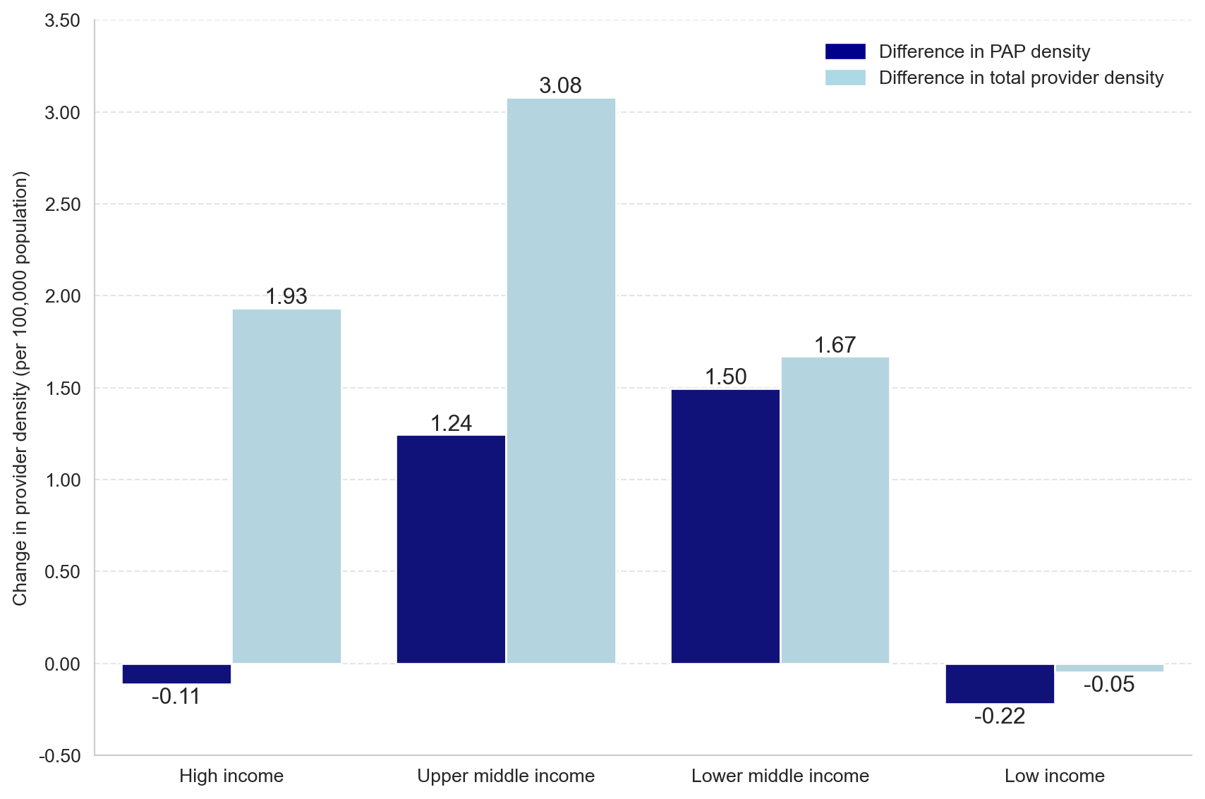
Figure 3
Plotly
Code
incomeorder = ['High income', 'Upper middle income','Lower middle income','Low income']t1 = px.bar(wbc, x='wbincome', y=['totalpap_capdiff','totalproviders_cap_diff'], barmode='group', labels={'variable':""}, template='plotly_white', text_auto=True, color_discrete_sequence=['darkblue','lightblue']).update_layout( xaxis_title='', xaxis_categoryorder='array', xaxis_categoryarray=incomeorder, yaxis_title='Change in providers per 100,000 people', legend=legendict, width=1000, height=600, template='plotly_white').update_traces(texttemplate='%{y:.2f}')t1.update_yaxes(showline=True, ticksuffix=" ").update_xaxes(showline=True)labeldict={'totalpap_capdiff':'Difference in PAP density', 'totalproviders_cap_diff':'Difference in total provider density'}for trace in t1['data']: trace['name'] = labeldict[trace['name']]#t1.write_image('figures/fig3 - pap_and_totalprovider_cap_diff.jpg', width=1000, height=562, scale=3, engine='kaleido')t1
Seaborn
Code
import matplotlib.pyplot as pltimport matplotlib.patches as mpatchesimport seaborn as snsimport pandas as pdsns.set_style("whitegrid")# Define the income order for x-axisincome_order = ['High income', 'Upper middle income', 'Lower middle income', 'Low income']# Melt the data to convert it to long formatwbc_melted = wbc.melt(id_vars='wbincome', value_vars=['totalpap_capdiff', 'totalproviders_cap_diff'])# Reorder the DataFrame based on 'income_order'wbc_melted['wbincome'] = pd.Categorical(wbc_melted['wbincome'], categories=income_order, ordered=True)wbc_melted = wbc_melted.sort_values('wbincome')# Create a grouped bar plot using catplotg = sns.catplot(x='wbincome', y='value', hue='variable', data=wbc_melted, kind='bar', palette={'totalpap_capdiff': 'darkblue', 'totalproviders_cap_diff': 'lightblue'}, height=6, aspect=1.5, legend_out=False)# Set axis labels and titlesg.set_axis_labels('', 'Change in provider density (per 100,000 population)')g.set_yticklabels([f'{tick:.2f}'for tick in g.ax.get_yticks()])# Remove top and right spinessns.despine(right=True, top=True)# Add grid lines for the y-axisg.ax.yaxis.grid(linestyle='--', alpha=0.5)# Set plot title and tighten layoutplt.tight_layout()# Add value labels to the barsfor p in g.ax.patches[:8]: height = p.get_height() width = p.get_width() x, y = p.get_xy() value = height if height >=0else height -0.13# Adjust the vertical alignment for negative values g.ax.annotate(f'{height:.2f}', (x + width /2, y + value), ha='center', va='bottom', fontsize=12)# Custom legend with colors matching the bar colorslegend_patches = [ mpatches.Patch(color='darkblue', label='Difference in PAP density'), mpatches.Patch(color='lightblue', label='Difference in total provider density')]g.ax.legend(handles=legend_patches, loc='upper right', bbox_to_anchor=(0.99, 0.99), frameon=False)# Save the figureplt.savefig('figures/fig3 - pap_and_totalprovider_cap_diff.jpg', dpi=1200)# Display the figureplt.show()
#to change the order of regions for this particular figureregionlist = ['European Region','Region of the Americas','Western Pacific Region', 'Eastern Mediterranean Region','South-East Asia Region','African Region']
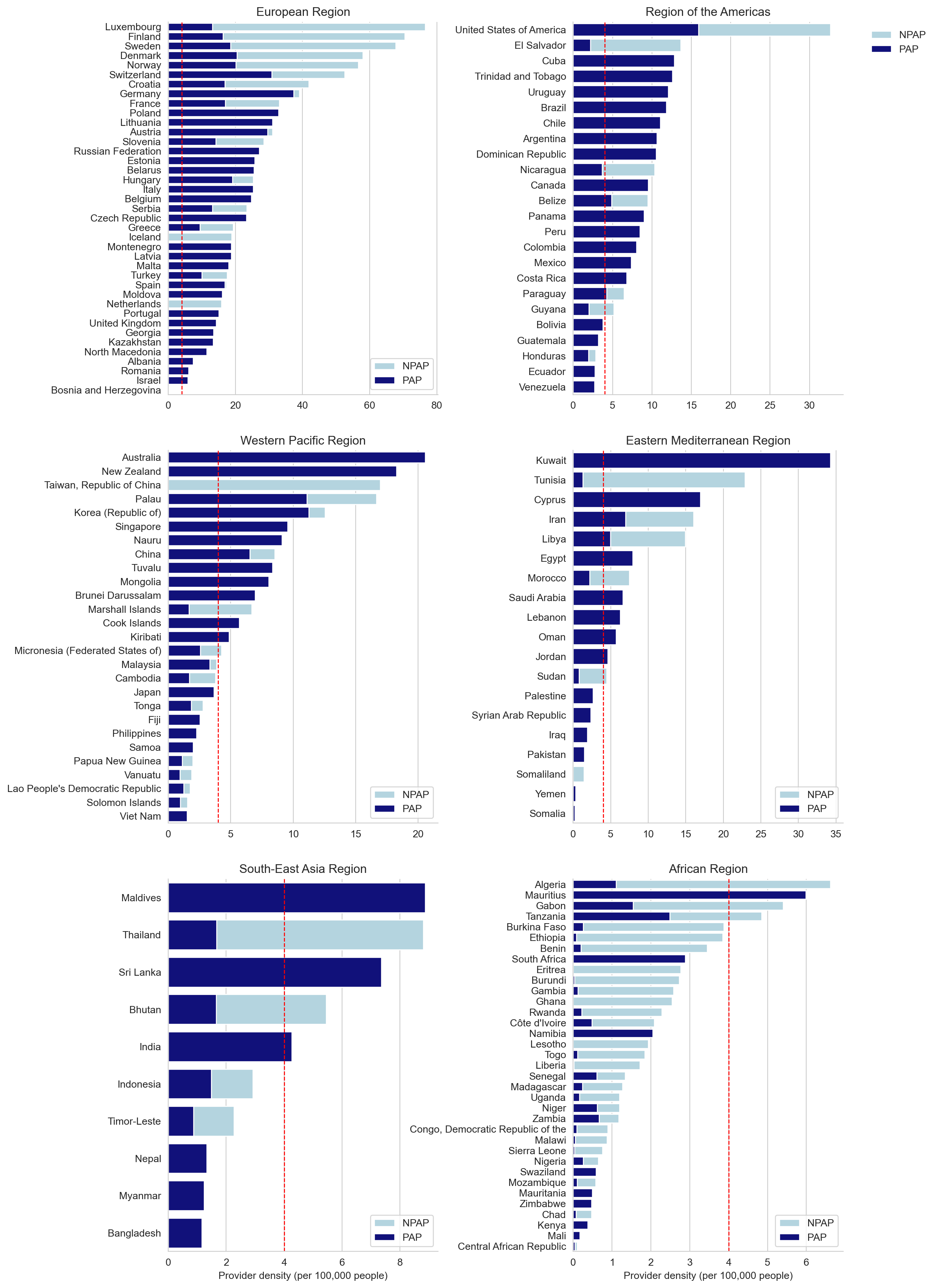
t1 = px.bar(dfg[dfg['Region_x']=='Region of the Americas'], x='country', y=['totalpap_cap','totalnpap_cap'], labels={'variable':""}, title='Total anesthesia providers per 100,000 population (PAP and NPAP)', color_discrete_sequence=['darkblue','lightblue']).update_layout( xaxis_categoryorder='total descending', yaxis_title='Total providers per 100,000', xaxis_title='')labeldict={'totalpap_cap':'PAP', 'totalnpap_cap':'NPAP'}for trace in t1['data']: trace['name'] = labeldict[trace['name']]#t1.write_image('americas_pap_npap.jpg', width=1000, height=500, scale=3, engine='kaleido')t1
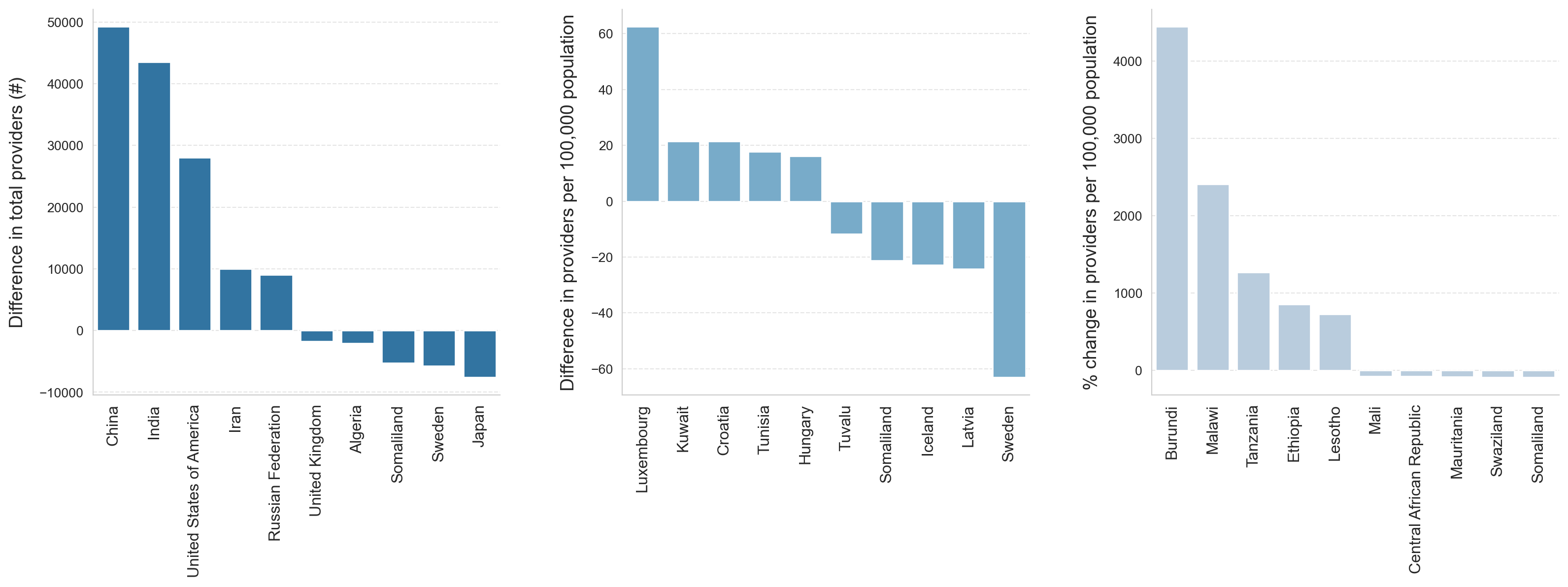
Figure 4
Code
subplots = make_subplots(rows=1, cols=3, horizontal_spacing=0.07)#,#subplot_titles=['Absolute difference in total providers (#)', 'Difference in total provider density','Percentage change in <br> total provider density (percent)'])def addcustomplot(var): data = dfg[((dfg[var].notnull()) & (dfg[var] != np.inf))].sort_values(by=[var], ascending=False).head() data = pd.concat([data, dfg[dfg[var].notnull()].sort_values(by=[var], ascending=False).tail()]) fig = go.Bar(x=data['country'], y=data[var])return figt1 = dfg[dfg['country']=='North Macedonia']['totalprovidersdiffpct']#plot 1subplots.add_trace(addcustomplot('totalprovidersdiff'), row=1,col=1)subplots.update_yaxes(title_text='Difference in total providers (#)').update_traces(marker=dict(color='#1f77b4'), row=1, col=1)#plot 2subplots.add_trace(addcustomplot('totalproviders_cap_diff'), row=1,col=2)subplots.update_yaxes(title_text='Difference in provider density', row=1,col=2).update_traces(marker=dict(color='#6baed6'), row=1, col=2)#plot 3subplots.add_trace(addcustomplot('totalproviders_cap_pct'), row=1,col=3)subplots.update_yaxes(title_text='% change in provider density', row=1, col=3).update_traces(marker_color='#b3cde3', row=1, col=3)#subplots.update_layout(title='Top and bottom changes in providers (absolute, per capita, and percent change)')subplots.update_layout(template='plotly_white', showlegend=False, width=1750, height=600, margin=dict(l=20, r=20, t=20, b=20))(subplots.update_xaxes(tickangle=270, tickfont=dict(size=16), linecolor='lightgray') .update_yaxes(showgrid=True, tickfont_size=1, title_font_size=20, title_standoff=0, linecolor='lightgray', linewidth=1))#subplots.write_image('figures/fig 4 - diff_metrics plotly.jpg', engine='kaleido', scale=3)subplots
as 2x2 grid
Code
# import matplotlib.pyplot as plt# import seaborn as sns# import numpy as np# sns.set_style("whitegrid")# # Your custom function modified for Seaborn# def addcustomplot(df, var, ax, y_label, plot_color):# data = df[((df[var].notnull()) & (df[var] != np.inf))].sort_values(by=[var], ascending=False).head()# data = data.append(df[df[var].notnull()].sort_values(by=[var], ascending=False).tail())# plot = sns.barplot(x='country', y=var, data=data, ax=ax, palette=[plot_color])# plot.set(xlabel=None) # remove the x axis label "country"# plot.set(ylabel=y_label) # use the current subplot titles as y axis labels# plot.yaxis.label.set_fontsize(12) # Increase y-axis label font size# for item in plot.get_xticklabels(): # rotate x labels for better fit# item.set_rotation(90)# item.set_fontsize(12) # Increase x-axis label font size# return ax# # Set up the subplot structure with a 2x2 grid, but we will only use three of these# fig, axes = plt.subplots(nrows=2, ncols=2, figsize=(15, 15), gridspec_kw={'height_ratios': [1, 1], 'hspace': 0.5, 'wspace': 0.2})# # Add your plots and increase y axis label font size# # Define custom colors to match the desired shades# darkblue = '#1f77b4' # Equivalent to Plotly's 'darkblue'# middleblue = '#6baed6' # A middle shade of blue# lightblue = '#b3cde3' # Equivalent to Plotly's 'lightblue'# colors = [darkblue, middleblue, lightblue]# addcustomplot(dfg, 'totalprovidersdiff', axes[0, 0], 'Difference in total providers (#)', colors[0])# addcustomplot(dfg, 'totalproviders_cap_diff', axes[0, 1], 'Difference in provider density', colors[1])# addcustomplot(dfg, 'totalproviders_cap_pct', axes[1, 0], '% change in provider density', colors[2])# for i in range(2):# for j in range(2):# axes[i, j].get_yaxis().get_label().set_fontsize(14)# axes[i, j].yaxis.labelpad = 10 # Increase space between y-axis label and the grid# axes[i, j].grid(axis='y', linestyle='--', alpha=0.5) # Add gridlines for y-axis# # Remove the top and right side borders of the plots# for ax in axes.flat:# ax.spines['top'].set_visible(False)# ax.spines['right'].set_visible(False)# # Remove the unused subplot# fig.delaxes(axes[1, 1])# # Adjust bottom margin to make space for x-axis labels# plt.subplots_adjust(bottom=.2)# # Tight layout often produces nice results# # It adjusts subplot params so that subplots are nicely fit in the figure# plt.tight_layout()# # Save your figure# plt.savefig('figures/fig 4 - diff_metrics.jpg', dpi=300, bbox_inches='tight')# # Display the figure# plt.show()
as 3x1 grid
Code
############################ make into 1 rowimport matplotlib.pyplot as pltimport seaborn as snsimport numpy as npsns.set_style("whitegrid")# Your custom function modified for Seaborndef addcustomplot(df, var, ax, y_label, plot_color): data = df[((df[var].notnull()) & (df[var] != np.inf))].sort_values(by=[var], ascending=False).head() data = pd.concat([data, dfg[dfg[var].notnull()].sort_values(by=[var], ascending=False).tail()]) plot = sns.barplot(x='country', y=var, data=data, ax=ax, palette=[plot_color]) plot.set(xlabel=None) # remove the x axis label "country" plot.set(ylabel=y_label) # use the current subplot titles as y axis labels plot.yaxis.label.set_fontsize(12) # Increase y-axis label font sizefor item in plot.get_xticklabels(): # rotate x labels for better fit item.set_rotation(90) item.set_fontsize(12) # Increase x-axis label font sizereturn ax# Set up the subplot structure with a 2x2 grid, but we will only use three of thesefig, axes = plt.subplots(nrows=1, ncols=3, figsize=(20, 6), gridspec_kw={'wspace': 0.3})# Add your plots and increase y axis label font size# Define custom colors to match the desired shadesdarkblue ='#1f77b4'# Equivalent to Plotly's 'darkblue'middleblue ='#6baed6'# A middle shade of bluelightblue ='#b3cde3'# Equivalent to Plotly's 'lightblue'colors = [darkblue, middleblue, lightblue]addcustomplot(dfg, 'totalprovidersdiff', axes[0], 'Difference in total providers (#)', colors[0])addcustomplot(dfg, 'totalproviders_cap_diff', axes[1], 'Difference in providers per 100,000 population', colors[1])addcustomplot(dfg, 'totalproviders_cap_pct', axes[2], '% change in providers per 100,000 population', colors[2])for i inrange(3): axes[i].get_yaxis().get_label().set_fontsize(14) axes[i].yaxis.labelpad =10# Increase space between y-axis label and the grid axes[i].grid(axis='y', linestyle='--', alpha=0.5) # Add gridlines for y-axis# Remove the top and right side borders of the plotsfor ax in axes.flat: ax.spines['top'].set_visible(False) ax.spines['right'].set_visible(False)# Remove the unused subplot#fig.delaxes(axes[1, 1])# Adjust bottom margin to make space for x-axis labelsplt.subplots_adjust(bottom=.2)# Tight layout often produces nice results# It adjusts subplot params so that subplots are nicely fit in the figureplt.tight_layout()# Save your figureplt.savefig('figures/fig 4 - diff_metrics.jpg', dpi=1200, bbox_inches='tight')# Display the figureplt.show()
Response rate
There are 6 possible groups of responses:
UN member countries, contacted responded
UN member countries, contacted, didn’t respond
UN member countries, did not contact
non UN member countries, contacted, responded
non UN member countries, contacted, didn’t respond
non UN member countries, did not contact
Code
df2['Email'] = df2.apply(lambda y: np.nan if y['Email']==""else y['Email'], axis=1)df2['Home Country'] = df2.apply(lambda x: np.nan if x['Home Country']==""else x['Home Country'], axis=1)
templist = ['Bosnia and Herzegovina','Niue','Somaliland','Taiwan, Republic of China','Tokelau']for i in templist: df['code3'] = df.apply(lambda x: 'nil'if x['country'] == i else x['code3'], axis=1)
Code
#countries with responses are those with total providers >1countrieswithresponses = df[df['totalproviders']>0][['country','code3']]# UN countries with responses are those countries with responses, that are also in the UN listun['response'] = un.apply(lambda x: "Has data"if x['allmembers'] in countrieswithresponses['country'].tolist() else'Have no data', axis=1)nodata = un['response'].str.contains('Have no data')# for those countries in the UN list with NO responses, do we have emails for them?un.loc[nodata,'response'] = un.loc[nodata].apply(lambda x: "No data, contacted"if x['allmembers'] in df2.query('Email.notnull()')['Home Country'].tolist() else"No data, not contacted", axis=1)un
# what are the places with responses that aren't in the UN list?countrieswithresponses[~countrieswithresponses['country'].isin(un['allmembers'].tolist())]['country'].value_counts()
country
Palestine                    3
Taiwan, Republic of China    1
Cook Islands                 1
Somaliland                   1
Niue                         1
Tokelau                      1
Name: count, dtype: int64
Code
# are there places with responses that aren't in the contact list!?countrieswithresponses[~countrieswithresponses['country'].isin(df2['Home Country'].tolist())]
country
code3
144
Somaliland
nil
Code
# are there countries in the contact list that aren't in the un list?print('these are all non-countries')df2[~df2['Home Country'].isin(un['allmembers'].tolist())]['Home Country'].value_counts()
these are all non-countries
Home Country
Taiwan, Republic of China    3
West Africa                  2
Palestine                    2
Kosovo                       2
French Polynesia             2
Hong Kong                    2
Republika Srpska             1
Aruba                        1
Bermuda                      1
Puerto Rico                  1
Cook Islands                 1
Niue                         1
Tokelau                      1
Name: count, dtype: int64
Code
# places in the contact list, that aren't countries, that dont have responsesdf2[df2['Email'].notnull() &~df2['Home Country'].isin(un['allmembers'].tolist()) &~df2['Home Country'].isin(countrieswithresponses['country'].tolist())]['Home Country'].value_counts()
Home Country
Kosovo              2
French Polynesia    2
Hong Kong           2
West Africa         1
Republika Srpska    1
Puerto Rico         1
Name: count, dtype: int64
In summary:
Code
print('There are 193 UN member countries')print('Of these, we have data from ',un['response'].value_counts()['Has data'],' of them')print('Of the countries with no data, we had contact information and tried to contact ',un['response'].value_counts()['No data, contacted'], 'of them')print('Of the countries with no data, we lacked contact information for',un['response'].value_counts()['No data, not contacted'], 'of them')print('We also have data from places that are not countries')print('There are',len(countrieswithresponses[~countrieswithresponses['country'].isin(un['allmembers'].tolist())]['country'].value_counts()), 'responses from those')# what about non countries that we attempted to contact?
There are 193 UN member countries
Of these, we have data from  149  of them
Of the countries with no data, we had contact information and tried to contact  23 of them
Of the countries with no data, we lacked contact information for 21 of them
We also have data from places that are not countries
There are 6 responses from those
How many countries w/ providers <5
Code
# realcountries is the countries from dfg that are present in the df called 'un', which is a csv of un member countries# necessary to exclude those answers that aren't real countriesrealcountries = dfg.loc[dfg['code3'].isin(un['code3'].value_counts().index)]
Code
# number of countries w/ pap <5len(realcountries[realcountries['totalpap_cap']<5])
75
Code
# number of countries w/ total prov <5len(realcountries[realcountries['totalproviders_cap']<5])
are there any countries with data that are not in the country verification list? Shouldn’t be - the verification list should contain all the countries with data, and whether or not they need to be verified.
# i'm so sorry this has to be done but bosnia has a response to OTHER_1 providers, so it's included in the groupby, but NOT included in the countries with responses!# so it should really be deleted from dfg. dfg should have been defined as countries with responses.dfg=dfg[~dfg['country'].str.contains('Bosnia')]dfg['verification_status'].value_counts().sum()
155
Code
len(countrieswithresponses.value_counts().index)
155
total number of countries is 156 because I deleted bosnia in dfg earlier, see comment
Code
df['country'].value_counts()
country
Morocco      4
Croatia      4
Austria      4
Slovenia     3
Zambia       3
            ..
Swaziland    1
Namibia      1
Jordan       1
Gambia       1
Senegal      1
Name: count, Length: 156, dtype: int64
data = dfg.groupby(by='wbincome').mean(numeric_only=True)[['totalgender','totalpap_gender','totalnpap_gender']]data2 = dfg.groupby(by='Region_x').mean(numeric_only=True)[['totalgender','totalpap_gender','totalnpap_gender']]
gendercols = ['totalpap_gender','totalnpap_gender','totalgender']genderlabels = ['PAPs','NPAPs','All providers']table_str='''<table class='table-style'> <thead> {# ######## FIRST MAKE THE COLUMNS IN THE HEADER ######### #} {# ######## THE COLUMNS ######### #} <tr class='darkgray'> <td></td> {% for i in genderlabels %} <td class='left-solid'>{{i}} </td> {% endfor %} </tr> </thead> <tbody> {# ######## NOW MAKE THE BODY ######### #} {# ######## FIRST SECTION ######### #} <tr class='section-break'><td colspan = 4> Income Group </td> </tr> {# ######## START EACH ROW WITH A LABEL ######### #} {% for i in data.index %} <tr> <td> {{i}} </td> {# ######## NOW EACH COLUMN FOR THAT ROW FROM THE DATAFRAME ######### #} {% for j in gendercols %} <td class='left-solid'> {{ data.at[i,j]|int }} </td> {% endfor %} </tr> {% endfor %} {# ######## Second SECTION ######### #} <tr class='section-break'><td colspan = 4> Region </td> </tr> {# ######## START EACH ROW WITH A LABEL ######### #} {% for i in data2.index %} <tr> <td> {{i}} </td> {# ######## NOW EACH COLUMN FOR THAT ROW FROM THE DATAFRAME ######### #} {% for j in gendercols %} <td class='left-solid'> {{ data2.at[i,j]|int }} </td> {% endfor %} </tr> {% endfor %} </tbody></table></html>'''template=Template(table_head+table_str)withopen('table_gender.html', "w") as text_file:print(template.render(data=data, data2=data2, genderlabels=genderlabels, gendercols=gendercols), file=text_file)#PUT ALL YOUR VARIABLES IN HEREHTML(template.render(data=data, data2=data2, genderlabels=genderlabels, gendercols=gendercols))
PAPs
NPAPs
All providers
Income Group
High income
43
63
48
Upper middle income
43
35
42
Lower middle income
36
39
37
Low income
30
35
31
Region
African Region
29
38
32
Eastern Mediterranean Region
34
51
35
European Region
51
67
54
Region of the Americas
48
52
48
South-East Asia Region
40
25
36
Western Pacific Region
33
36
35
Code
t1 = px.scatter(dfg, x='country',y='totalgender', color='wbincome', template='plotly_white', labels={'wbincome':'Income group','totalgender':'% of providers who are women','country_shr':"Country"}, category_orders={'wbincome':incomeorder}).update_layout(xaxis_categoryorder='total descending', legend_orientation='h',legend_y=1.1)t1.write_image('prop_women.jpg', width=1000, height=500, scale=2, engine='kaleido')t1